Draw a Segment in a Circle

Draw Circle — Diameter, Radius, Arc and Segment Using Python Matplotlib Module

In this blog, we will plot indicate at origin and so circle. Later on that we will plot diameter, radius, arc and segment(chord) using Matplotlib library.

Created by Nutan

Data about circles

Circumvolve

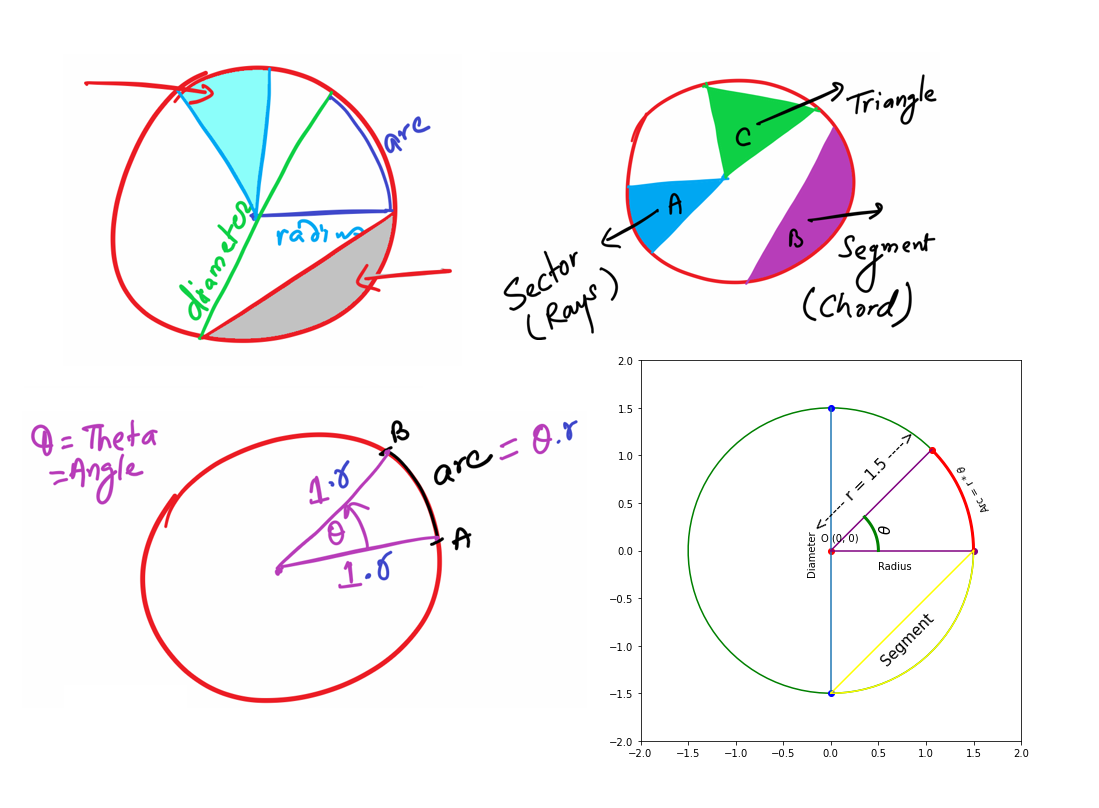
A circle is a shape consisting of all points in a plane that are at a given distance from a given betoken, the middle; equivalently information technology is the bend traced out past a point that moves in a aeroplane so that its distance from a given signal is constant. The distance between any point of the circle and the center is chosen the radius.

Circumference

The distance around the circle.

Center

The signal equidistant from all points on the circle.

Diameter

Diameter a line segment whose endpoints lie on the circle and that passes through the eye; or the length of such a line segment. This is the largest distance between any 2 points on the circle.

Radius

The distance between any signal of the circle and the center is called the radius.

Arc

whatsoever continued part of a circle. Specifying two end points of an arc and a heart allows for two arcs that together make up a full circumvolve.

Chord

A line segment whose endpoints lie on the circle, thus dividing a circle into two segments.

Import Modules

                      import matplotlib.pyplot as plt
import numpy every bit np
from numpy import sin, cos, pi, linspace                  

Plot signal at origin(0, 0)

                      #draw bespeak at origin (0, 0)
plt.plot(0,0, color = 'red', marker = 'o')
plt.testify()                  

Output:

Point at origin(0, 0)

Add together annotation and fix xlim and ylim

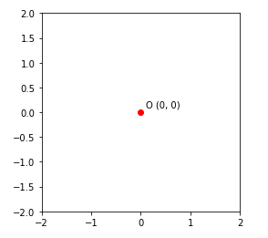
          #describe point at origin (0, 0)
plt.plot(0,0, color = 'red', marker = 'o')
            plt.gca().comment('O (0, 0)', xy=(0 + 0.1, 0 + 0.1), xycoords='data', fontsize=10)                                plt.xlim(-ii, 2)
plt.ylim(-two, 2)
plt.gca().set_aspect('equal')            
plt.show()        

Output:

Indicate with annotaion

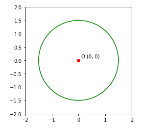
Draw a circumvolve

          #draw bespeak at origin (0, 0)
plt.plot(0,0, color = 'scarlet', marker = 'o')
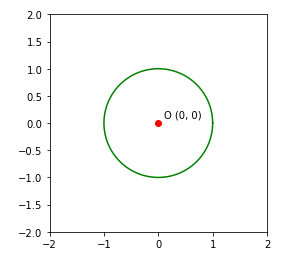
plt.gca().annotate('O (0, 0)', xy=(0 + 0.1, 0 + 0.1), xycoords='information', fontsize=10)                      #draw a circle
angles = linspace(0 * pi, 2 * pi, 100 )                                xs = cos(angles)
ys = sin(angles)                                plt.plot(xs, ys, color = 'light-green')                    plt.xlim(-two, 2)
plt.ylim(-2, 2)
plt.gca().set_aspect('equal')
plt.show()        

Output:

Cicle

Increment circle radius from 1 to 1.five

          plt.plot(0,0, color = 'ruby-red', marker = 'o')
plt.gca().comment('O (0, 0)', xy=(0 + 0.1, 0 + 0.1), xycoords='information', fontsize=ten)          #draw a circle
angles = linspace(0 * pi, 2 * pi, 100 )
            r = ane.5
xs = r * cos(angles)
ys = r * sin(angles)                    plt.plot(xs, ys, color = 'dark-green')          plt.xlim(-2, ii)
plt.ylim(-2, 2)
plt.gca().set_aspect('equal')
plt.show()        

Output:

Circle with radius one.5

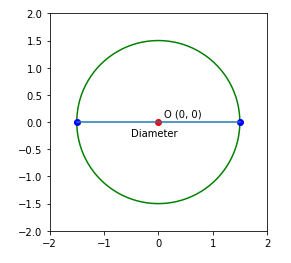
Draw diameter of circumvolve

          #draw point at orgin
plt.plot(0,0, color = 'red', marking = 'o')
plt.gca().annotate('O (0, 0)', xy=(0 + 0.1, 0 + 0.one), xycoords='data', fontsize=ten)          #draw a circle
angles = linspace(0 * pi, 2 * pi, 100 )
r = 1.v
xs = r * cos(angles)
ys = r * sin(angles)          plt.plot(xs, ys, colour = 'green')                      #draw daimeter
plt.plot(1.5, 0, marker = 'o', color = 'blue')
plt.plot(-1.5, 0, marker = 'o', color = 'bluish')
plt.plot([ane.5, -1.5], [0, 0])
plt.gca().annotate('Diameter', xy=(-0.v, -0.25), xycoords='information', fontsize=10)                    plt.xlim(-2, ii)
plt.ylim(-2, two)
plt.gca().set_aspect('equal')
plt.show()        

Output:

Diameter

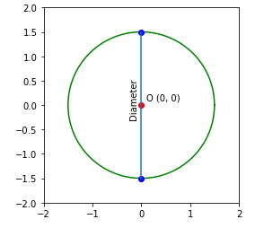
Describe bore from xc degree

          #draw betoken at orgin
plt.plot(0,0, colour = 'red', marker = 'o')
plt.gca().comment('O (0, 0)', xy=(0 + 0.1, 0 + 0.ane), xycoords='information', fontsize=10)          #draw circle
angles = linspace(0 * pi, 2 * pi, 100 )
r = 1.5
xs = r * cos(angles)
ys = r * sin(angles)          plt.plot(xs, ys, colour = 'green')          #depict daimeter
            plt.plot(0, 1.5, marking = 'o', color = 'blue')
plt.plot(0, -1.5, mark = 'o', color = 'blue')
plt.plot([0, 0], [1.5, -1.5])
plt.gca().annotate('Diameter', xy=(-0.25, -0.25), xycoords='information', fontsize=10, rotation = ninety)                    plt.xlim(-two, 2)
plt.ylim(-2, 2)
plt.gca().set_aspect('equal')
plt.show()        

Output:

Bore

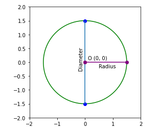
Describe radius

          #draw point at orgin
plt.plot(0,0, color = 'red', marker = 'o')
plt.gca().annotate('O (0, 0)', xy=(0 + 0.1, 0 + 0.i), xycoords='data', fontsize=ten)          #draw circumvolve
r = one.five
angles = linspace(0 * pi, ii * pi, 100 )
xs = r * cos(angles)
ys = r * sin(angles)          plt.plot(xs, ys, color = 'green')          #depict daimeter
plt.plot(0, ane.5, marker = 'o', color = 'blue')
plt.plot(0, -ane.5, mark = 'o', colour = 'blue')
plt.plot([0, 0], [i.5, -1.5])
plt.gca().annotate('Diameter', xy=(-0.25, -0.25), xycoords='data', fontsize=10, rotation = 90)                      #draw radius
plt.plot(0, 0, marker = 'o', colour = 'imperial')
plt.plot(1.5, 0, mark = 'o', colour = 'purple')
plt.plot([0, 1.5], [0, 0], colour = 'purple')
plt.gca().annotate('Radius', xy=(0.5, -0.two), xycoords='data', fontsize=10)                    plt.xlim(-two, 2)
plt.ylim(-ii, 2)
plt.gca().set_aspect('equal')
plt.show()        

Output:

Radius

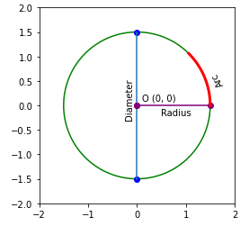
Describe arc from 0 to pi/4

          #draw point at orgin
plt.plot(0,0, color = 'reddish', marker = 'o')
plt.gca().comment('O (0, 0)', xy=(0 + 0.1, 0 + 0.ane), xycoords='data', fontsize=ten)          #draw circumvolve
r = 1.5
angles = linspace(0 * pi, 2 * pi, 100 )
xs = r * cos(angles)
ys = r * sin(angles)          plt.plot(xs, ys, color = 'green')          #describe daimeter
plt.plot(0, i.5, marker = 'o', color = 'bluish')
plt.plot(0, -one.5, marking = 'o', color = 'blueish')
plt.plot([0, 0], [one.5, -1.five])
plt.gca().annotate('Bore', xy=(-0.25, -0.25), xycoords='data', fontsize=x, rotation = 90)          #draw radius
plt.plot(0, 0, marker = 'o', color = 'majestic')
plt.plot(1.5, 0, marker = 'o', colour = 'purple')
plt.plot([0, 1.five], [0, 0], color = 'purple')
plt.gca().annotate('Radius', xy=(0.5, -0.2), xycoords='data', fontsize=10)                      #draw arc
arc_angles = linspace(0 * pi, pi/4, 20)
arc_xs = r * cos(arc_angles)
arc_ys = r * sin(arc_angles)
plt.plot(arc_xs, arc_ys, color = 'red', lw = three)
plt.gca().annotate('Arc', xy=(1.five, 0.4), xycoords='data', fontsize=x, rotation = 120)                    plt.xlim(-ii, ii)
plt.ylim(-two, 2)
plt.gca().set_aspect('equal')
plt.show()        

Output:

Arc

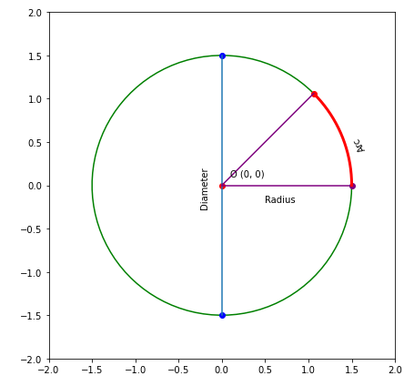
Draw radius from 0 to pi/4 and consummate the arc

          plt.figure(figsize = (18, 7))          #describe point at orgin
plt.plot(0,0, colour = 'red', mark = 'o')
plt.gca().annotate('O (0, 0)', xy=(0 + 0.i, 0 + 0.i), xycoords='data', fontsize=10)          #draw circle
r = 1.5
angles = linspace(0 * pi, 2 * pi, 100 )
xs = r * cos(angles)
ys = r * sin(angles)          plt.plot(xs, ys, color = 'green')          #describe daimeter
plt.plot(0, 1.5, marker = 'o', color = 'blue')
plt.plot(0, -1.v, marker = 'o', color = 'blue')
plt.plot([0, 0], [1.five, -1.5])
plt.gca().annotate('Bore', xy=(-0.25, -0.25), xycoords='data', fontsize=x, rotation = 90)          #draw radius
#plt.plot(0, 0, marker = 'o', color = 'regal')
plt.plot(1.five, 0, marker = 'o', color = 'majestic')
plt.plot([0, 1.five], [0, 0], colour = 'majestic')
plt.gca().annotate('Radius', xy=(0.five, -0.2), xycoords='information', fontsize=ten)          #draw arc
arc_angles = linspace(0 * pi, pi/four, 20)
arc_xs = r * cos(arc_angles)
arc_ys = r * sin(arc_angles)
plt.plot(arc_xs, arc_ys, color = 'ruddy', lw = 3)
plt.gca().annotate('Arc', xy=(1.5, 0.iv), xycoords='data', fontsize=10, rotation = 120)                      #draw another radius
plt.plot(r * cos(pi /4), r * sin( pi / four), marker = 'o', color = 'red')
plt.plot([0, r * cos(pi /four)], [0, r * sin( pi / 4)], color = "purple")                    plt.xlim(-ii, two)
plt.ylim(-ii, 2)
plt.gca().set_aspect('equal')
plt.show()        

Output:

Arc

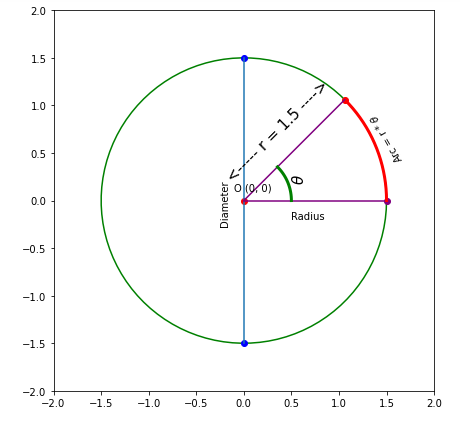
Write annotation of arc

          plt.figure(figsize = (eighteen, 7))          #draw point at orgin
plt.plot(0,0, color = 'scarlet', marker = 'o')
plt.gca().comment('O (0, 0)', xy=(0 - 0.i, 0 + 0.i), xycoords='information', fontsize=10)          #describe circumvolve
r = 1.five
angles = linspace(0 * pi, 2 * pi, 100 )
xs = r * cos(angles)
ys = r * sin(angles)          plt.plot(xs, ys, color = 'greenish')          #describe daimeter
plt.plot(0, one.5, mark = 'o', color = 'blue')
plt.plot(0, -ane.5, marking = 'o', color = 'blue')
plt.plot([0, 0], [one.5, -1.5])
plt.gca().annotate('Diameter', xy=(-0.25, -0.25), xycoords='data', fontsize=10, rotation = 90)          #draw radius
#plt.plot(0, 0, marker = 'o', color = 'purple')
plt.plot(1.5, 0, marker = 'o', colour = 'royal')
plt.plot([0, 1.5], [0, 0], color = 'majestic')
plt.gca().annotate('Radius', xy=(0.5, -0.ii), xycoords='data', fontsize=10)          #draw arc
arc_angles = linspace(0 * pi, pi/iv, twenty)
arc_xs = r * cos(arc_angles)
arc_ys = r * sin(arc_angles)
plt.plot(arc_xs, arc_ys, color = 'reddish', lw = 3)
            #plt.gca().annotate('Arc', xy=(1.5, 0.4), xycoords='data', fontsize=x, rotation = 120)
plt.gca().annotate(r'Arc = r * $\theta$', xy=(i.3, 0.4), xycoords='data', fontsize=ten, rotation = 120)                    #draw some other radius
plt.plot(r * cos(pi /4), r * sin( pi / 4), marker = 'o', colour = 'red')
plt.plot([0, r * cos(pi /4)], [0, r * sin( pi / 4)], colour = "purple")                      # depict theta angle and notation
r1 = 0.5
arc_angles = linspace(0 * pi, pi/4, xx)
arc_xs = r1 * cos(arc_angles)
arc_ys = r1 * sin(arc_angles)
plt.plot(arc_xs, arc_ys, colour = 'green', lw = iii)
plt.gca().annotate(r'$\theta$', xy=(0.5, 0.2), xycoords='data', fontsize=15, rotation = 90)
plt.gca().annotate('<----- r = ane.5 ---->', xy=(0 - 0.2, 0 + 0.2), xycoords='data', fontsize=15, rotation = 45)                    plt.xlim(-ii, two)
plt.ylim(-2, 2)
plt.gca().set_aspect('equal')
plt.show()        

Output:

Arc with annotation

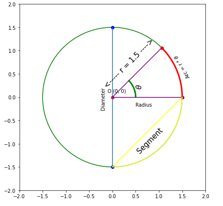
Describe segment(chord)

          plt.figure(figsize = (18, seven))          #draw indicate at orgin
plt.plot(0,0, colour = 'red', mark = 'o')
plt.gca().annotate('O (0, 0)', xy=(0 - 0.one, 0 + 0.1), xycoords='data', fontsize=10)          #depict circumvolve
r = 1.5
angles = linspace(0 * pi, 2 * pi, 100 )
xs = r * cos(angles)
ys = r * sin(angles)          plt.plot(xs, ys, color = 'green')          #draw daimeter
plt.plot(0, 1.5, marker = 'o', color = 'bluish')
plt.plot(0, -ane.5, marker = 'o', color = 'blue')
plt.plot([0, 0], [1.5, -1.five])
plt.gca().annotate('Diameter', xy=(-0.25, -0.25), xycoords='information', fontsize=10, rotation = 90)          #describe radius
#plt.plot(0, 0, marker = 'o', color = 'majestic')
plt.plot(1.5, 0, marker = 'o', color = 'purple')
plt.plot([0, 1.5], [0, 0], color = 'majestic')
plt.gca().annotate('Radius', xy=(0.v, -0.2), xycoords='data', fontsize=10)          #describe arc
arc_angles = linspace(0 * pi, pi/4, xx)
arc_xs = r * cos(arc_angles)
arc_ys = r * sin(arc_angles)
plt.plot(arc_xs, arc_ys, color = 'carmine', lw = 3)
#plt.gca().annotate('Arc', xy=(one.v, 0.iv), xycoords='data', fontsize=10, rotation = 120)
plt.gca().annotate(r'Arc = r * $\theta$', xy=(1.3, 0.iv), xycoords='data', fontsize=10, rotation = 120)          #draw another radius
plt.plot(r * cos(pi /iv), r * sin( pi / 4), marking = 'o', color = 'ruby')
plt.plot([0, r * cos(pi /4)], [0, r * sin( pi / 4)], colour = "purple")          # draw theta bending and annotation
r1 = 0.v
arc_angles = linspace(0 * pi, pi/iv, 20)
arc_xs = r1 * cos(arc_angles)
arc_ys = r1 * sin(arc_angles)
plt.plot(arc_xs, arc_ys, color = 'light-green', lw = 3)
plt.gca().annotate(r'$\theta$', xy=(0.five, 0.two), xycoords='data', fontsize=fifteen, rotation = xc)
plt.gca().annotate('<----- r = 1.5 ---->', xy=(0 - 0.2, 0 + 0.2), xycoords='data', fontsize=15, rotation = 45)                      #draw segment
r2 = 1.5
segment_angles = linspace(three/4 * 2* pi, ii * pi, 100 )
segment_xs = r2 * cos(segment_angles)
segment_ys = r2 * sin(segment_angles)                                plt.plot(segment_xs, segment_ys, color = 'yellowish')                                plt.plot([1.five, 0], [0, -ane.5], colour = 'xanthous')
plt.gca().annotate('Segment', xy=(0.5, -ane.ii), xycoords='data', fontsize=15, rotation = 45)
seg_x_p1 = r2 * cos(2 * pi)                    plt.xlim(-two, 2)
plt.ylim(-two, 2)
plt.gca().set_aspect('equal')
plt.evidence()        

Output:

Segment(chord)

That'south it. Thanks for reading.

pharrpheine.blogspot.com

Source: https://medium.com/@nutanbhogendrasharma/draw-circle-diameter-radius-arc-and-segment-using-python-matplotlib-module-343705417622